MomentumRNN: Integrating Momentum into Recurrent Neural Networks

What is MomentumRNN about?

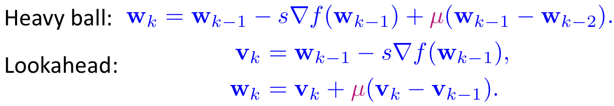
We develop a gradient descent (GD) analogy of the recurrent cell. In particular, the hidden state update in a recurrent cell is associated with a gradient descent step towards the optimal representation of the hidden state. We then integrate momentum that used for accelerating gradient dynamics into the recurrent cell, which results in the momentum cell as shown in Figure 1. At the core of the momentum cell is the use of momentum to accelerate the hidden state learning in RNNs. We call the RNN that consists of momentum cells the MomentumRNN [1].

Here are our research paper, slides, lighting talk, and code.

Figure 1: Comparison between the momentum-based cells and the recurrent cell.

Why does MomentumRNN matter?

The major advantages of MomentumRNN are fourfold:

  • MomentumRNN can alleviate the vanishing gradient problem in training RNN.
  • MomentumRNN accelerates training and improves the accuracy of the baseline RNN.
  • MomentumRNN is universally applicable to many existing RNNs.
  • The design principle of MomentumRNN can be generalized to other advanced momentum-based optimization methods, including Adam [2] and Nesterov accelerated gradients with a restart [3, 4].

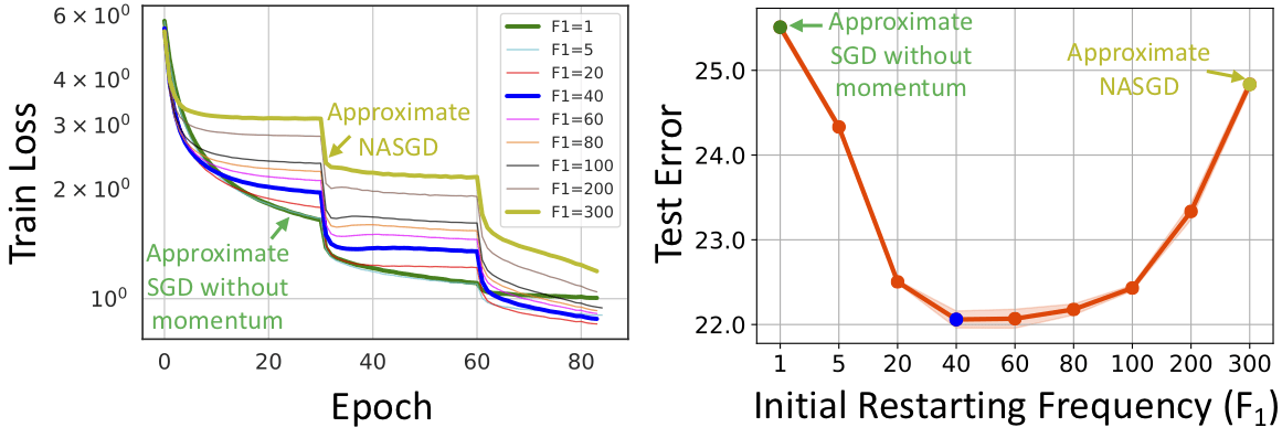
Why does MomentumRNN have a principled approach?

First, let us review the hidden state update in RNN as given in the following equation.

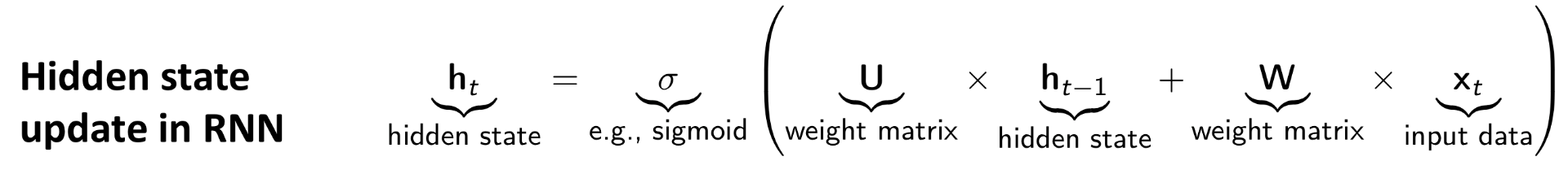
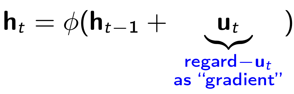
In order to incorporate momentum into an RNN, we first interpret that the input data at time t provides a gradient for updating the hidden state at time t – 1. In particular, let us consider the following re-parameterization of the hidden state update equation.

The recurrent cell can then be re-written as:

Adding momentum to the recurrent cell yields

LetWe get the following momentum cell

Momentum cell is derived from the momentum update for gradient descent, and thus, it is principled with theoretical guarantees provided by the momentum-accelerated dynamical system for optimization. Similar derivation can be employed to derive other momentum-based cells from state-of-the-art optimization methods, such as the Adam cell, the RMSProp cell, and the Nesterov accelerated gradient cells as illustrated in Figure 1.

Furthermore, applying backpropagation-through-time on the MomentumRNN, we can show that

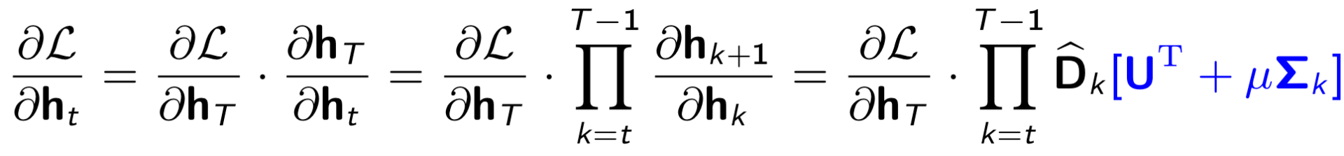
According to the above equation, choosing a proper momentum constant μ in MomentumRNN helps alleviate the vanishing gradient problem.

Why is MomentumRNN simple?

Implementing momentum cells only requires changes in a few lines of the recurrent cell code. Also, our momentum-based principled approach can be integrated into LSTM and other RNN models easily.

Does MomentumRNN work?

1. Our momentum-based RNNs outperform the baseline RNNs on a variety of tasks across different data modalities. Below we show our empirical results on (P)MNIST and TIMIT tasks. Results for other tasks can be found in our paper.

Figure 2: Momentum-based LSTMs outperform the baseline LSTMs on (P)MNIST image classification and TIMIT speech recognition tasks.

2. Our momentum-based approach can be applied to the state-of-the-art RNNs to improve their performance. Below we consider the orthogonal RNN equipped with dynamic trivialization (DTRIV) as a baseline and show that our MomentumDTRIV still outperforms the baseline DTRIV on PMNIST and TIMIT tasks.

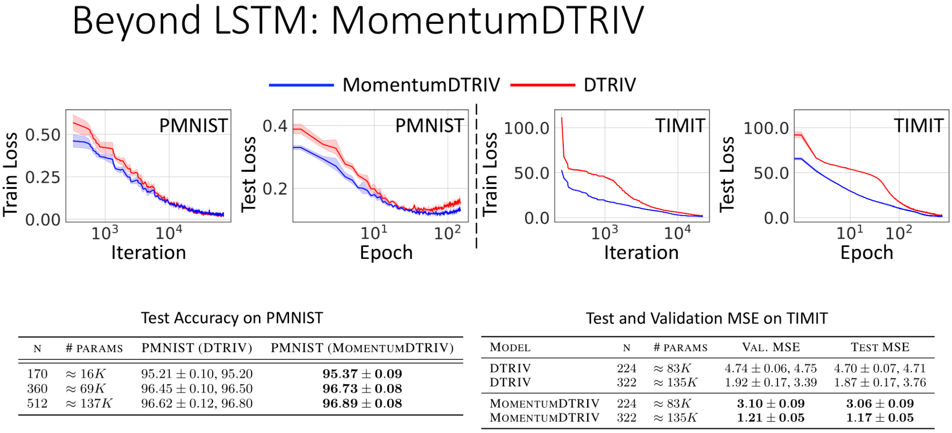
Figure 3: Our momentum approach helps improve the performance of the state-of-the-art orthogonal RNN equipped with dynamic trivialization (DTRIV).

3. Momentum-based RNNs are much more efficient than the baseline RNNs. Figure 4 shows that momentum-based RNNs require much less time to reach the same test accuracy as the corresponding RNNs.

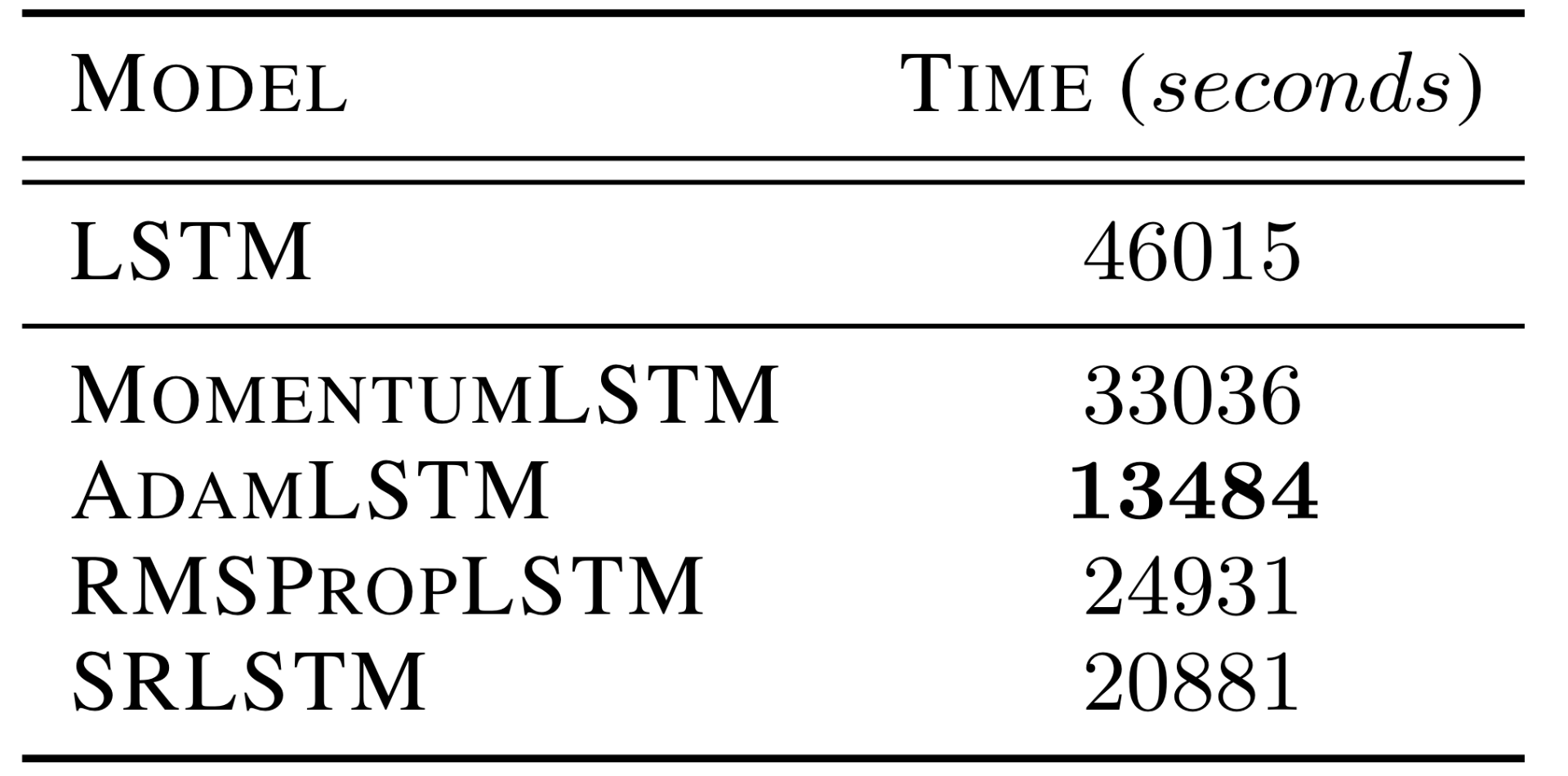
Figure 4: Total computation time to reach the same 92.29% test accuracy of LSTM for PMNIST classification task.

References

1. Tan Nguyen, Richard G Baraniuk, Andrea L Bertozzi, Stanley J Osher, and Bao Wang. MomentumRNN: Integrating Momentum into Recurrent Neural Networks. In Advances in Neural Information Processing Systems, 2020.

2. Diederik P Kingma and Jimmy Ba. Adam: A method for stochastic optimization. arXiv preprint arXiv:1412.6980, 2014.

3. Yurii E Nesterov. A method for solving the convex programming problem with convergence rate o (1/kˆ 2). In Dokl. Akad. Nauk Sssr, volume 269, pages 543–547, 1983.

4. Bao Wang, Tan M Nguyen, Andrea L Bertozzi, Richard G Baraniuk, and Stanley J Osher. Scheduled restart momentum for accelerated stochastic gradient descent. arXiv preprint arXiv:2002.10583, 2020.


Scheduled Restart Momentum for Accelerated Stochastic Gradient Descent

What is Scheduled Restart Stochastic Gradient Descent (SRSGD) about?

Stochastic gradient descent (SGD) with constant momentum and its variants such as Adam are the optimization algorithms of choice for training deep neural networks (DNNs). Since DNN training is incredibly computationally expensive, there is great interest in speeding up convergence. Nesterov accelerated gradient (NAG) improves the convergence rate of gradient descent (GD) for convex optimization using a specially designed momentum; however, it accumulates error when an inexact gradient is used (such as in SGD), slowing convergence at best and diverging at worst. In this post, we’ll briefly survey the current momentum-based optimization methods and then introduce the Scheduled Restart SGD (SRSGD), a new NAG-style scheme for training DNNs. SRSGD replaces the constant momentum in SGD by the increasing momentum in NAG but stabilizes the iterations by resetting the momentum to zero according to a schedule. Using a variety of models and benchmarks for image classification, we demonstrate that, in training DNNs, SRSGD significantly improves convergence and generalization. Furthermore, SRSGD reaches similar or even better error rates with fewer training epochs compared to the SGD baseline. (Check out the research paper, slides, and code.)

Why does SRSGD have a principled approach?

Gradient descent (GD) has low computational complexity, is easy to parallelize, and achieves a convergence rate independent of the dimension of the underlying problem. However, it suffers from the pathological curvature, regions of the loss surface which are not scaled properly. In particular, in those areas, the surface is very steep in one direction but flat in other directions. As a result, as shown in Figure 1, GD is bouncing the ridges of the ravine, slowing down the convergence of the algorithm.

Figure 1: Pathological Curvature. GD bounces the ridges of the ravine along one direction and moves slowly in another direction [A. Kathuria, 2018].

Pathological curvature problem can be avoided with second-order methods, such as the Newton’s method, which take into account the curvature of the loss surface. However, those method require the Hessian, which is costly to compute. Momentum-based method is an alternative approach, which approximately captures the curvature by considering the past behavior of the gradients. In momentum-based methods, previous gradients are added into the current gradients in an exponential average manner as follow [B. Polyak, 1964]:

As shown in Figure 2 below, when adding up the gradients, the components along the bouncing direction are zeroed out while the components which lead to the local minima are enforced. Therefore, momentum helps speed up the local convergence of GD.

Figure 2: Momentum adds up the component along w2 while zeroing out components along w1, thereby canceling the bouncing between the two ridges [A. Kathuria, 2018].

While heavy ball and lookahead momentums improve the local convergence. They do not provide global guarantees and the convergence rate is still O(1/k). Nesterov accelerated gradient descent (NAG) improves the convergence rate to O(1/k2)  by increasing the momentum at each step as follows [Y. E. Nesterov, 1983]:

It can be proven that the exact limit of NAG scheme by taking small step size s is a 2nd-order ODE, thus NAG is not really a descent method, but inherits the oscillatory behavior from its ODE counterpart (See Figure 3 left) [W. Su, S. Boyd, and E. Candes, 2014].

Figure 3: Comparison between GD, GD + Momentum, NAG, ARNAG, and SRNAG in the case of exact gradient, constant variance Gaussian noise corrupted gradient, and decaying variance Gaussian noise corrupted gradient. The objective function in this case study is convex.

Adaptive Restart NAG (ARNAG) improves upon NAG by reseting the momentum to zero whenever the objective loss increases, thus canceling the oscillation behavior of NAG [B. O’donoghue, 2015]. Under a proper sharpness assumption, ARNAG can achieve an exponential convergence rate [V. Roulet et al., 2017].

Unfortunately, when the gradients are inexact, as in the case of Stochastic Gradient Descent (SGD), both NAG and ARNAG fail to obtain fast convergence. While NAG accumulates error and converges slowly or even diverges, ARNAG is restarted too often and almost degenerates to the SGD without momentum. Under inexact gradient setting, restarting the Nesterov Momentum in NAG according to a fixed schedule helps overcome the error accumulation and high-frequent restarting issues (see Figure 3 middle, right). This approach results in the Scheduled Restart NAG (SRNAG) [V. Roulet et al., 2017]. The update of SRNAG is given by

Our Scheduled Restart SGD (SRSGD) is the stochastic version of SRNAG for training with mini-batches

An interesting interpretation of SRSGD is that it is an interpolation between SGD without momentum (when the restart frequency is small) and SGD with Nesterov Momentum (NASGD) (when the restart frequency is large) (see Figure 4).

Figure 4: Training loss and test error of ResNet-101 trained on ImageNet with different initial restarting frequencies F1. We use linear schedule and linearly decrease the restarting frequency to 1 at the last learning rate. SRSGD with small F1 approximates SGD without momentum, while SRSGD with large F1 approximates NASGD.

Why is SRSGD simple?

SRSGD has no additional computational or memory overhead. Furthermore, implementing SRSGD only requires changes in a few lines of the SGD code. Thus, SRSGD inherits all the computation advantages of SGD: low computational complexity and easy to parallelize.

Does SRSGD work?

1. DNNs trained by SRSGD generalize significantly better than those trained by SGD with constant momentum. The improvement becomes more significant as the network grows deeper (see Figure 5).

Figure 5: Error vs. depth of ResNet models trained with SRSGD and the baseline SGD with constant momemtum. Advantage of SRSGD continues to grow with depth.

2. SRSGD reduces overfitting in very deep networks such as ResNet-200 for ImageNet classification.

3. SRSGD can significantly speed up DNN training. For image classification, SRSGD can significantly reduce the number of training epochs while preserving or even improving the network’s accuracy. In particular, on CIFAR10/100, the number of training epochs can be reduced by half with SRSGD while on ImageNet the reduction in training epochs ranges from 10 to 30 and increases with the network’s depth (see Figure 6).

Figure 6: Test error vs. number of epoch reduction in CIFAR10 and ImageNet training. The dashed lines are test errors of the SGD baseline. For CIFAR, SRSGD training with fewer epochs can achieve comparable results to SRSGD training with full 200 epochs. For ImageNet, training with less epochs slightly decreases the performance of SRSGD but still achieves comparable results to the SGD baseline training.

References

Kathuria, A. Intro to optimization in deep learning: Momentum, RMSProp, and Adam. https://blog.paperspace.com/intro-to-optimization-momentum-rmsprop-adam/.

Nesterov, Y. E. A method for solving the convex programming problem with convergence rate o (1/kˆ 2). In Dokl. akad. nauk Sssr, volume 269, pp. 543–547, 1983.

O’donoghue, B. and Candes, E. Adaptive restart for accelerated gradient schemes. Foundations of computational mathematics, 15(3):715–732, 2015.

Polyak, B. T. Some methods of speeding up the convergence of iteration methods. USSR Computational Mathematics and Mathematical Physics, 4(5):1–17, 1964.

Roulet, V. and d’Aspremont, A. Sharpness, restart and acceleration. In Advances in Neural Information Processing Systems, pp. 1119–1129, 2017.

Su, W., Boyd, S., and Candes, E. A differential equation for modeling nesterov’s accelerated gradient method: Theory and insights. In Advances in Neural Information Processing Systems, pp. 2510–2518, 2014.